Understanding and implementing Bayes Factor/Bayes Hypothesis testing

Bayes Factor (BF) is a quantity for the evidence in observed data to support one model against another, where the two models are usually a “null”/$M_1$ vs an “alternative”/$M_2$. If you don’t like to read the maths, jump to 1.2 for an intuitive example.

1. What is Bayes Factor?
2. When is BF useful / Why do you need it?
3. Some implementations
- 3.1 A straightforward implementation in R
- 3.2 Laplace’s method
4. Take-home messages
References

1. What is Bayes Factor?

1.1 Some definitions

The mathematical definition of BF is

\[B(x) = \frac{p(M_1|X)}{p(M_2|X)} \cdot \frac{p(M_2)}{p(M_1)}\]

The insight here is that BF is the ratio of posterior odds for $M_1$ to the prior odds for $M_1$. However, this is not how you compute BF; if you want to compute BF, you need to do an integral like this

\[B(x) = \frac{ \int_{\Theta_1} p(X|\theta) p(\theta | M_1) d\theta }{ \int_{\Theta_2} p(X|\theta) p(\theta | M_2) d\theta }\]

..which is a weighted sum of likelihoods $p(X|\theta)$ under a specified $p(\theta|M_k), k \in {1,2}$. This is because the posterior odds itself is defined by $B(x)$.

\[\frac{p(M_1|X)}{p(M_2|X)} = \frac{ \int_{\Theta_1} p(M_1) p(X|\theta) p(\theta | M_1) d\theta }{ \int_{\Theta_2} p(M_2) p(X|\theta) p(\theta | M_2) d\theta }\]

So in order to compute the posterior odds, you have to integrate over the prior parameter distribution to compute BF first. In inspecting the target integral, you might have already noticed that the function being integrated is very similar to the posterior density of the parameters, i.e. $p(\theta|X)=p(X|\theta)p(\theta) / p(X)$, except for minor differences like the lack of the normalizing constant $p(X)$ and conditioning on a specified model $M_k$. This is exactly the insight we will use for approximating the integral using Laplace’s method, which we will cover in the implementation section.

1.2 One example

I really like the example presented in here. Below I will re-write this example , but in a simpler context. Credits of the original example should go to the original author(s).

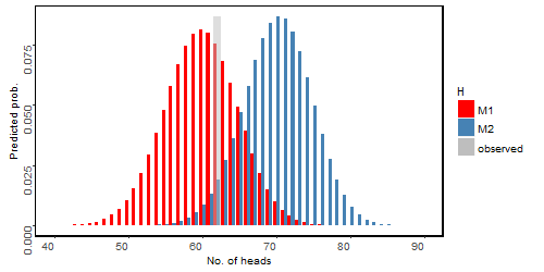
In analogy to this excellent example, I will make up an unfair coin tossing example similarly. Suppose we have an uneven coin that tends to land on heads. Two people hold different views about the uneveness. Connie believes the probability of head is 70%, while Frank believes its more even, only 60%. They tossed the coin 100 times and observed 62 were heads. Apparently the observation is more close to Frank’s prediction, but Connie argues that 62 is also possible under her model, and so her hypothesis cannot be ruled out. We can plot Frank and Connie’s predicted probabilities as below:

It does seem obvious that the data favors Frank’s model, but by how much? Given this plot, we can easily see that under Frank’s hypothesis, the probability of y=62 is 0.075, while it is ~0.02 under Connie’s hypothesis. Assuming a Binomial distribution of the observed heads $y=62$, we can compute BF as

\[\frac{p(y|H_f)}{p(y|H_c)} = \frac{0.0753}{0.0191} = 3.95\]

In R, we can write this line as

N=100; y=62
p.frank=0.6; p.connie=0.7
dbinom(y, N, p.frank)/dbinom(y, N, p.connie)
## [1] 3.953

This means the observed data is around 4 times more likely in Frank’s hypothesis compared to Connie’s.

In real-world situations, it is quite rare that we could have such specific predictions. More likely, each people will also have a subjective distribution to represent their beliefs – or, being “Bayesian”. Let’s assume that Frank now assumes $\theta \sim trunc N(0.6, \tau_1^2), \tau_1=0.2$, that is, Frank is not very sure about his prediction; while Connie assumes $\theta \sim trunc N(0.7, \tau_2^2), \tau_2=0.1$, she is confident that the parameter is around 0.7. Note that we intentionally did not choose Binomial distribution’s conjugate prior, Beta; because I believe except for the stylistic examples you learn from Stats classes, most cases encountered in real problems don’t have such conjugacy. And I will show you how to handle such non-conjugacy in “implementation” section.

For now let’s first take a look as the prior distribution of $\theta$ (top panel) and the predicted probability for each possible $y$ (bottom panel) in the figure below:

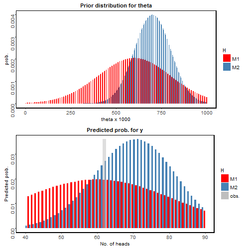
Wow! Now the observation (grey) favors Connie’s prediction (blue). How does that happen?

It is because Frank has a relatively large uncertainty about his prediction. His prediction of $\theta$ is “flat”; he predicted the value of theta could very well range from 0 to 1, although it does peak around 0.6. On the other hand, Connie has a high confidence in her prediction around $\theta=0.7$. We can again compute the BF in this case:

\[B(x) =\frac{p(y|H_f)}{p(y|H_c)} = \frac{0.0196}{0.0271} = 0.722\]

It seems Connie and Frank’s predictions are similarly plausible given the observed data, though observation is slightly leaning towards Connie. Can we go a bit further for interpretation?

1.3 Interpretations

So far, we have covered basic definitions of BF and a very intuitive but still informative example, let’s move on for some interpretations – such that even if you still don’t know how to compute/code a BF, you know what it means. Being regarded as the Bayesian alternative for Frequentist hypothesis testing, or rather, p-value, BF also has some empirical thresholds to catalog the significance, proposed by Jeffereys:

Bayes Factor	Strength of Evidence
B <= (1/10)	Strong against M1
(1/10) < B <= (1/3)	Substantial against M1
(1/3) < B < 1	Barely against M1
1 <= B < 3	Barely for M1
3 <= B < 10	Substantial for M1
B >= 10	Strong for M1

Apparently these thresholds are heuristics. But in the above example, we can say that in the first scenario, the observed data is “substantial for M1”; while in the second scenario, the observed data is “barely against M1” due to the large uncertainty in prior distribution.

2. When is BF useful / Why do you need it?

Compared to Frequentist hypothesis testing, there are several advantages. You might want to consider BF over likelihood ratio test if you fit into one or more of the following listings: A) You can actually accept the null hypothesis; while in hypothesis testing, you can only “fail to reject null hypothesis” but cannot accept the null. In fact, in BF there is no null or alternative at all so that two competing models are completely interchangeable.

B) The tested two models don’t have to be nested. In the hypothesis testing, the two models have to be either $H_0: \theta = 0$ vs. $H_1: \theta \neq 0$, or $H_0: \theta \leq 0$ vs. $H_1: \theta >0$. While in BF, as demonstrated in the above example, the two models can be very flexible.

3. Some implementations

3.1 A straightforward implementation in R

Now let’s figure out some implementations to compute BF in R. If you still remember in the first part, to compute BF we need to integrate to marginalize out the parameters. We first compile the function we want to integrate:

binom_norm_pdf = function(theta, stuff)
# theta: parameter to be integrate
# stuff: a list consists of N, y, p, tau
{
N = stuff$N
y = stuff$y
p = stuff$p
tau = stuff$tau
dbinom(y, size=N, prob=theta, log=F) *
dnorm(theta, mean=p, sd=tau)/(pnorm(1, mean=p, sd=tau)-pnorm(0, mean=p, sd=tau))
}

Very straightforward, right? You can write any prior to this binomial parameters – but remember to truncate it outside of 0 to 1, i.e the normalizing constant.

Next we need a wrapper function to do the integral for us. Fortunately, most programming languages now provide a simple and useful numerical approximation function to do integration. Check out the documentations for integration in R and python. Below is a wrapper in R. A side note: how about double integral? In python one can use “dblquad”; in R one might try “cubature” package (I have never used this one myself). Either way, for multi-dimensional integral beyond double integral, one should try Monte-carlo integration.

bayes.factor =function(p1, p2, tau1, tau2, N, y)
# a wrapper for computing bayes factor of binomial with truncated normal prior
# p: prior mean; tau: prior standard deviation
# N: total trials; y: No. of successes
{
m1=integrate(binom_norm_pdf, 0, 1, stuff=list(N=N, y=y, p=p1, tau=tau1))
m2=integrate(binom_norm_pdf, 0, 1, stuff=list(N=N, y=y, p=p2, tau=tau2))
m1$value / m2$value
}

And we can do some testing to see if it works as expected:

# reproduce the example, second scenario in the first section
bayes.factor(0.6, 0.7, 0.2, 0.1, 100, 62)
### 0.722
# shrink the variance to approximate the first scenario
bayes.factor(0.6, 0.7, 0.01, 0.01, 100, 62)
### 3.726

3.2 Laplace’s method

Yet another way to compute the integral is by Laplacian approximation.My gut feeling is that Laplace’s method could be numerically more stable. If you know the answer and/or have some experimental results, please let me know!

The way Laplacian approximation works is very clearly demonstrated here. Below I just copy-paste a simple example for using Laplacian approximation in LearnBayes package in R. This example is from this link.

# computing bayes factors

# write a new function to faciliate the comparison of two models

bayes.factor <- function(model1, model2){
require(LearnBayes)
fit1 <- laplace(model1$logpost, model1$mode, model1$stuff)
fit2 <- laplace(model2$logpost, model2$mode, model2$stuff)
log.bayes.factor <- fit1$int - fit2$int
print(paste('The log Bayes factor in support of model 1 over model 2 is',
round(log.bayes.factor, 2)))
}

# example
# compare two models
# M1: y is binomial(20, p), p is beta(3, 10)
# M2: y is binomial(20, p), p is beta(10, 3)
# observe y = 5

# write a log posterior
# (don't forget normalizing constants)

lbinomial.beta <- function(p, stuff){
y <- stuff$data[1]
n <- stuff$data[2]
a <- stuff$prior[1]
b <- stuff$prior[2]
dbinom(y, size=n, prob=p, log=TRUE) +
dbeta(p, a, b, log=TRUE)
}

# use bayes.factor function

model1 <- list(logpost=lbinomial.beta,
mode=0.5,
stuff=list(data=c(5, 20), prior=c(3, 10)))

model2 <- list(logpost=lbinomial.beta,
mode=0.5,
stuff=list(data=c(5, 20), prior=c(10, 3)))

bayes.factor(model1, model2)
Loading required package: LearnBayes
[1] "The log Bayes factor in support of model 1 over model 2 is 4.61"

# here we can compare approximate Bayes factor with exact value

log.pred1 <- log(pbetap(c(3, 10), 20, 5)) -
log(pbetap(c(10, 3), 20, 5))
round(log.pred1, 2)
[1] 4.61

4. Take-home messages

I hope you have a rough (or complete, hopefully) understanding of Bayes Factor once you reach to this point! Compile your own Bayes Factor Calculator now :)

Source code for this post can be fould in Github here.

References

**Disclaimer: The content in this post is my own understanding for Bayes factor, based on several online resourses. Please use with care. Comments/discussions are welcomed.